
GCP tutorial#
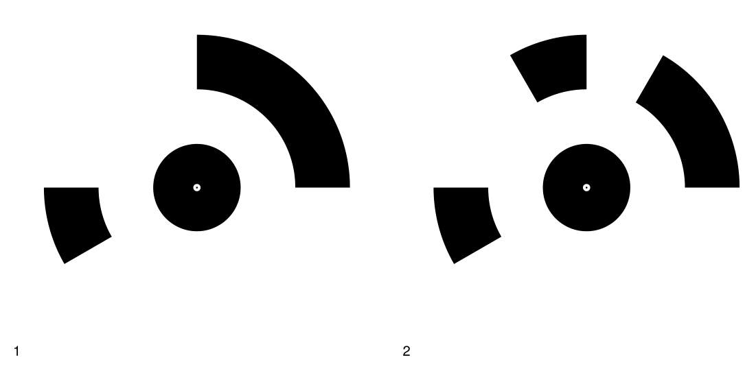
While other GCP marker types exist, we here focus on the use of either ArUco or Agisoft Metashape markers. Both marker types are of the binary fiducial sort, and, in principal, machine readable.
GCP generation and detection#
Slight differences exist in the way both are generated and detected, with Metashape markers strongly relying on the Metashape GUI and ArUco markers being mostly programming-based. Both, however, require well-established real world coordinates to be worth the effort.
Leave generated markers as-is
Most GCPs feature black-white markers. It is important to not change the white background colour, nor to remove white or black borders. These are needed for the automated detection of the markers, and are inherent to their correct functioning.
Real world coordinates#
As mentioned previously, real world coordinates should be measured consistently across all markers, i.e., always opt for the same measuring location and method of measurement.
Correct and systematic archiving of the locations is furthermore key to automisation later on. As part of the standardised project environment, it is therefore encouraged to format all GCP IDs and their corresponding real world coordinates in the following manner:
1,15.83193045,78.33763246,224.6672
2,15.83061642,78.33836842,221.3598
3,15.82920799,78.3390649,202.7514
4,15.82944846,78.33972477,184.2172
5,15.83092679,78.33907352,183.6924
6,15.83094077,78.33962431,164.2002
7,15.83085931,78.34003023,152.5401
8,15.82992376,78.34011196,169.7791
Herein the first column represents the GCP ID, followed by longitude, latitude, and altitude with the EPSG:4326 CRS. Once completed, make sure to save the file as a comma-separated-value (csv) file with name gcp_table.csv in the expected directory:
{project_directory}\data_directory\gcps\prepared\gcp_table.csv
Correct GCP IDs and order
Always make sure the GCP numbers in the gcp_table.csv file correspond with the actual GCP IDs. They should therefore always be unique (i.e., used only once).
Furthermore, be aware that the file uses longitude-latitude formatting as opposed to the common latitude-longitude order!
Agisoft Metashape#
To generate Metashape GCP markers, proceed to Tools/Markers/Print markers… to open the Print Markers dialog. Multiple parameters can be set, including the bit-encoding of the marker (Marker type); the Center point radius of the centre dot; how many markers to include per (Targets per page); and the Font size.
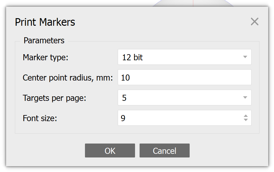
Fig. 36 Overview of the Metashape marker generation window.#
Centre dot size
When using Metashape markers, it is extremely important to chose an appropriate Center point radius, as it effectively determines the detectability of the marker. When the centre dot is no longer visible, Metashape will have great difficulty in automatically detecting the marker.
ArUco#
While the Metashape markers are exported all at once, more freedom is given to the generation of ArUco markers. Multiple options exist, ranging from online marker generators to the use of the popular OpenCV image processing suite, featuring both c++ and Python implementations.
One can even generate the ArUco markers from within the iFrame below:
Herein the Dictionary corresponds to the bit-encoding used by the Metashape markers. It is slightly more intuitive, however, as the {No}x{No} indicates the number of rows and columns of the marker. The Marker ID is a fixed identification number of a given marker within the same dictionary. Keep in mind, however, that markers from different dictionaries may have the same Marker ID, yet will have very different features! Finally, the Marker size determines the size of the marker. Make sure to pick an acceptable size.
Why not give it a shot yourself, and see how the markers change whilst you change the parameters?
Finally, you can save the marker by clicking open, and printing it as a PDF.
Programming approach
For those interested in using the programming approach, please read the OpenCV image processing suite article linked to above, as well as the example tutorial available at Scientific Python. This allows for far more freedom, including the automated generation of multiple markers in a circle as used for hand-sized sample digitisation.
GCP detection#
Compatible CRS
Always make sure to select a compatible CRS when dealing with markers. For instance, using metric measurements while in a longitude latitude CRS will give rise to very funky scaling issues! Probably wise to change the project or marker CRS to EPSG:9001 (Local Coordinates (m)) when dealing with metric measurements. Do so by right-clicking the active chunk in the Workspace, and then select Reference Settings….
Manual detection#
In order to manually detect GCPs, one first has to create a new Agisoft Metashape project and import all the taken images. Then one can browse through the images and manually look through all the images for the GCP markers. Once identified, proceed by right clicking on the point of interest to open the marker dialog. Here, one can either place a new marker, or choose to place a previously-added marker.
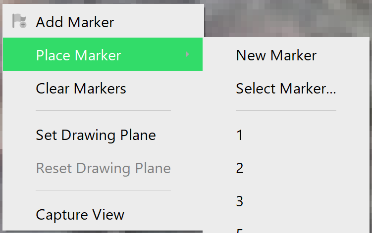
Fig. 37 Dialog for adding or placing specific markers. Be advised: one can only place specific markers after having added them previously.#
When added, a green flag appears that can be moved around by click-holding the left mouse button. This is especially useful for finetuning locations.
Once done, proceed to the Reference panel and find that the markers you added have been added to the project - albeit without real world positional values. Also shown are the number of projections, accuracy and error, of which the latter two also remain blank. Positional information can either be added directly into the Reference panel by double clicking one of the fields, as shown in Fig. 38, or by importing reference data.
Fig. 38 A marker with ID point 1 has been added to the project. Thusfar, no positional information is available, though the metadata shows that the marker has been identified in a single image (Projections). Editing the GCP point data can be easily done by double clicking each of the fields.#
Reference data is imported through the dialog opened by selecting File/Import/Import Reference…. Make sure to select the correct Coordinate System, select Comma as the Delimiter, and select the appropriate Columns for the Label, longitude, Latitude, and Altitude.
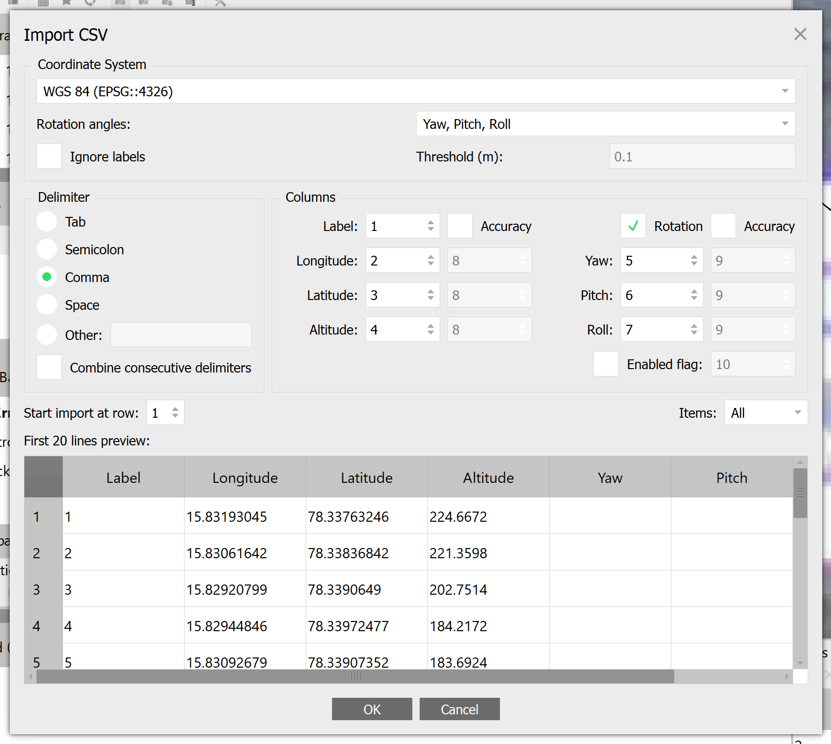
Fig. 39 Importing reference data for the GCP marker positions. Make sure to select the gcp_table.csv file when prompted.#
Matching labels
Make sure to double check and match all GCP IDs (=Labels) prior to importing. Rename the picked Labels in the Reference panel prior to importing, if you have to!
Automated detection#
A more significant difference exists in the way both marker types are automatically detected.
Metashape#
In Metashape, the Marker Detection dialog can be used to automatically detect the binary Metashape markers. This dialog can be accessed through Tools/Markers/Detect markers…. To optimise marker detection, it is advised to set the Marker type parameter equal to the bit-encoding selected during generation and leave the other parameters as-is before clicking OK to proceed.
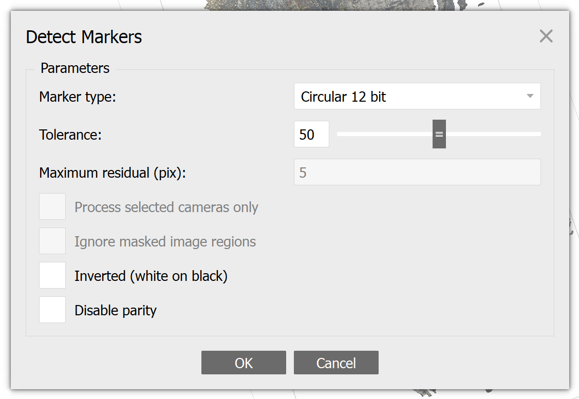
Fig. 40 Metashape GUI option for marker detection.#
ArUco#
Python installation required
The following steps require the installation of Python and the automated metashape scripts.
Prior to automated detection, we will have to configure a settings or parameter file for the automated metashape scripts.
Head over to the tutorial and put together a minimal working example (MWE) configuration consisting of:
minimal configuration parameters
Add photos
GCPs - detection
GCPs - add to project additional parameters
Make sure to place this file in the config directory of the standardised project environment.
Then proceed with the Python tutorial to subsequently add all images to the Metashape project; to detect the GCPs in all the images; to add the detected GCPs and corresponding real world coordinates to the Metashape project.