
Metashape Tutorial#
This tutorial (and exercise) features the following learning goals:
You will learn the basics of Agisoft Metashape
You will use Agisoft Metashape to digitise samples and/or outcrops
Support
Please note that we only provide feedback and support for students enrolled in the course at the University Centre of Svalbard.
3D model reconstruction with Agisoft Metashape#
Creating high-quality models the USGS way
The United States Geological Survey [] has put together an excellent tutorial on the use of Agisoft Metashape for creating high resolution digital elevation models. Although digital elevation models are but one of many desired products, the same guide can be used for the creation of high resolution and properly processed DOMs. USGS guidelines and the quick start guide to processing (Table 1) can be found here, and should be used supplementary to this tutorial.
https://pubs.usgs.gov/of/2021/1039/ofr20211039.pdf
In this session we will learn how to use Agisoft Metashape. This is an established SfM photogrammetry package and is often used in the Arctic Geology department at UNIS to create digital outcrop models (DOMs) and hand-sample models (HSMs). This session introduce basic processing through the graphical user interface through use of a standardised data set.
Software version
The following tutorial assumes the use of Agisoft Metashape version 2.x.x. Note that versions 1.6.x-1.8.x are very similar, and can use the same tutorials (though the interface and pop-up menus may be slightly different).
To see whether you are indeed running the correct version proceed to Help/About Metashape… in the menu bar. This should provide you with the major release, minor, and patch (2.0.x) version number, as well as the build.
If the version does not match the version listed above, please either
update the installation; or
contact the Seismic Lab software responsible (Peter Betlem)
Think before doing…
Always remember that quality comes at a cost, in this case as a computational cost (i.e., time) and storage cost (i.e., size).
In processing this is the key dilemma, and requires you to think about the output before you start.
Is it really necessary to generate a 500 GB model for a 1 by 1 square metre area, considering that your max upload limit for an assignment is only 200 MB?
Further reading
The guidelines below are based on the official Agisoft 3D model reconstruction tutorial. This tutorial, as well as more in-depth help, can be visited here.
A standardised project environment#
We will be using a standardised project environment throughout this course. It is recommended to use this setup (or something similar) throughout all future projects as well. The use of this standardised project setup is furthermore a requirement for digital models to be uploaded to the Svalbox DB.
Proceed by creating the following project_directory in the folder where you have all your projects.. Herein folders are named without extensions, and filenames are given extensions. Text between {} indicates variable names.
{project_directory} (The folder with all files related to this project)
|   overview_img.{ext}
|   description.txt
├───config (where you place your configuration files)
        {cfg_0001}.yml
        {cfg_0002}.yml
        ...
├───data (where you unzipped the files to)
├───────100MEDIA (The folder in which all the images reside)
|           {img_0001}.{ext}
|           {img_0002}.{ext}
|           ...
├───────101MEDIA (The folder in which all the images reside)
|           {img_0001}.{ext}
|           {img_0002}.{ext}
|           ...
|       ...
├───────199MEDIA (The folder in which all the images reside)
|           {img_0001}.{ext}
|           {img_0002}.{ext}
|           ...
├───────gcps
|           (We'll get back to this in a later session)
├───────GNSS
|           (We'll get back to this in a later session)
├───export (where you place export models and files to)
        ...
└───metashape (This is where you save your Agisoft Metashape projects to)
        {metashape_project_name}.psx
        .{metashape_project_name}.files
        {metashape_project_name}_processing_report.pdf
        (optionally: {metashape_project_name}.log)
{project_directory} (The folder with all files related to this project)
|   overview_img.{ext}
|   description.txt
├───config (where you place your configuration files)
        {cfg_0001}.yml
        {cfg_0002}.yml
        ...
├───data (where you unzipped the files to)
├───────f0001 (The folder with images acquired on the first flight)
|           {img_0001}.{ext}
|           {img_0002}.{ext}
|           ...
├───────f0002 (The folder with images acquired on the second flight)
|           {img_0001}.{ext}
|           {img_0002}.{ext}
|           ...
|       ...
├───────f9999 (The folder with images acquired on the last flight)
|           {img_0001}.{ext}
|           {img_0002}.{ext}
|           ...
├───────gcps
|           (We'll get back to this in a later session)
├───────GNSS
|           (We'll get back to this in a later session)
├───export (where you place export models and files to)
        ...
└───metashape (This is where you save your Agisoft Metashape projects to)
        {metashape_project_name}.psx
        .{metashape_project_name}.files
        {metashape_project_name}_processing_report.pdf
        (optionally: {metashape_project_name}.log)
The standardised project structures (as we will see later on) are important for automated processing and archiving. The project structures are identical in principle, only differing in the way images are sorted.
Photo set#
Having created the standardised project structure, proceed with extracting your taken images to the following directory:
{project_directory}\data\100MEDIA
{project_directory}\data\100MEDIA (includes up to 999 images)
{project_directory}\data\101MEDIA (includes remaining images)
{project_directory}\data\f0001
{project_directory}\data\f0002
{project_directory}\data\f0003
In case the image count exceeds 999 images, make sure to utilise multiple folders in the data_directory. While you are at it, why not sort the images by flight or acquisition to improve your data structure? For instance, those digitising hand-sized samples, or who have acquired data over multiple UAV flights, may find it beneficial to sort the data in specific ways. Not only is it easier to find the data that way, but it also prevents accidental data-overwrites of data with non-unique filenames!
Want to follow along without your own data?
Go ahead and download the package, then extract the archive’s contents as per the above.
URL:
Adding photos#
Next we’ll be adding the photos to Agisoft Metashape. This assumes To do this, proceed to and click on Add photos… from Workflow in the menu bar. In the dialog that pops up, browse to the project_directory/100MEDIA folder that you created in the previous section. Select all files to be processed. These should now show up in a chunk with cameras in the Workspace panel. Verify that this is indeed the case by double clicking one of the cameras in the Workspace/Chunk/Cameras panel.
Save often!
It is important to save your work often. Make a habit of saving at least after every step. To do so, proceed to Save as… under File in the menu bar, and save your project in the project_directory/metashape directory that you created when extracting in data.
Python console and sorting your project data#
As you may have noticed while adding your images, most cameras only allow for 999 unique file names (e.g., DJI001-DJI999). When hundreds of files are added to a single project, this can quickly become confusing. After all, did file DJI007 originate from flight 1 or from flight 2? It is thus important to store files in different subfolders (as previously described), but also to have those subfolders available within the processing project in Metashape. An easy way to do this is shown in Fig. 5. Right click the Images tab within the workspace, then click on Add Camera Group. Then select all cameras that belong to the same acquisition or flight and drag them into the new Camera Group.
Fig. 5 Creating image groups and sorting the input data of the project.#
Alternatively, as we will see in Session 4, we can automate most aspects of the workflow either by using Batch processing or by using the Metashape API. We here provide an example of how to use the Metashape API to quickly rename all photos within the project to reflect the data subdirectory they are in.
Proceed to the Console panel. If you cannot find it, go to the main menu bar, select View and click Console to activate it. This opens the terminal, and allows you to interact with the project through Python.
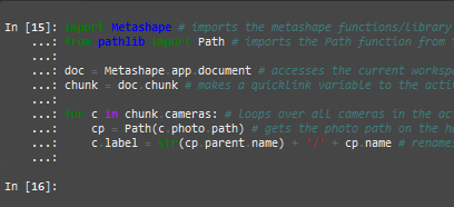
Fig. 6 View of the Python console in Metashape.#
Paste in the following script and see what happens with the labels of your files:
import Metashape # imports the metashape functions/library
from pathlib import Path # imports the Path function from the pathlib library

doc = Metashape.app.document # accesses the current workspace and document
chunk = doc.chunk # makes a quicklink variable to the active chunk in the document

for c in chunk.cameras: # loops over all cameras in the active chunk
    cp = Path(c.photo.path) # gets the photo path on the harddrive for each photo
    c.label = str(cp.parent.name) + '/' + cp.name # renames the camera label in the metashape workspace to reflect the parent directory of the photo
Analyze photos#
Before actual processing begins, we need to analyse the imported photos. This is done by right clicking any of the photos in a Chunk, then selecting Estimate Image Quality…, and select all photos to be analysed, as shown in Fig. 7.
Fig. 7 Estimating image quality in the Metashape GUI.#
One can then open the Photos pane by clicking Photos in the View menu. Then, make sure to view the details rather than icons to check the Quality for each image (Fig. 8.)
Fig. 8 Showing the image quality and disable photos that do not meet the requirement in the Metashape GUI.#
Then, filter on quality and Disable all selected cameras that do not meet the standard. Agisoft recommends a Quality of at least 0.5.
Masking photos#
When using pictures that have a non-neutral or messy background, Agisoft Megashape will likely try to identify common features (key and tie points) in the background. This will show up as tie points (blue) outside of your object on your images. This will become a problem if you move your object for a different halo or perspective. To mitigate this issue, you can select (mask) the areas of the photo that will not be analysed.
Double click on the image you want to mask.
Type Ctrl L or click on the selection tool. Choose tool based on your object and placement of the tie points (blue). a. Are the tie points far away from your object, the most effective tool might be the rectangle (as this is faster than the intelligent scissor tool). b. If your object is very dark compared to e.g. a white background you can also try the magic wand tool, but make sure it doesn’t select the tie points that lie within your object.
Right click and select invert mask and then add selection as shown in Fig. 9. The tie points that lie within the dark area will now be ignored when you align your photos again.
To apply the masks in the alignment of the photos (see next section), you can select apply masks to: keypoints in the advanced tab of the pop-up menu when aligning the photos. If you have already aligned your photos, but you have gone back and added masks, remember to check the Reset the current alignment box.
Fig. 9 Instructions on how to mask an object in the Metashape GUI.#
Aligning photos#
With the photos now imported into Metashape and analysed, we can proceed with the alignment process. This process goes through all images in the project and tries to identify common features. In Metashape this first requires the estimation of camera positions for each photo, which are then used to build a sparse cloud. Select Align Photos… in the Workflow menu.
A dialog will pop up with several parameter options. Most important here is the Accuracy parameter, which governs whether your photos are down-sampled before alignment.
For now we’ll skip the other parameters; just make sure to deselect Reference preselection, Guided image matching, and Adaptive camera model fitting. Keep Generic preselection and Exclude stationary tie points selected.
After clicking OK, Metashape starts aligning your photos. This may take a while, but assuming there is sufficient overlap between the data, a sparse point cloud will be shown on the screen (in the Model tab) once processing is done. If not, one can select this by clicking the four-dotted icon in the menu.
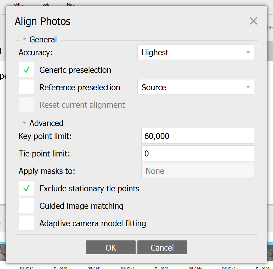
Fig. 10 The Align Photos dialog after opening it from the Workflow menu.#
Down-sampling
Down-sampling is the process in which you combine parts of a data set, resulting in the loss of knowledge. For example, down-sampling a 1000x1000 pixel image to a 100x100 image results in a factor 100 compression of data (= easier to process), but you also lose the initial resolution!
Depending on your computer specifications, you’ll have to weigh computational time versus output quality.
Give it a shot, and compare the photo alignment results with medium vs high processing accuracy.
Masking
If the alignment did not work or if the result looks bad, then it may help to apply masks to your input imagery. Please refer back to the masking step (Masking photos) on how to better apply masks and improve the alignment output.
Improve alignment step: Error Reduction-Optimization and Camera Calibration#
Ground control points
Additional steps are needed to ensure ground control points and checkpoints are adequately integrated into the model. We will discuss what ground control points are and what they can be used for in Ground control points (GCPs).
Those implementing ground control points, please refer to the USGS manual for the correct sequence of steps and optimizations.
Although the photos have now been aligned, it is important to further optimize the cameras. This is done by selecting Optimize Cameras from the Tools menu. A dialog will pop up with several parameter options pre-selected. Most important here is to at least select make sure that the Estimate tie point covariance is enabled.
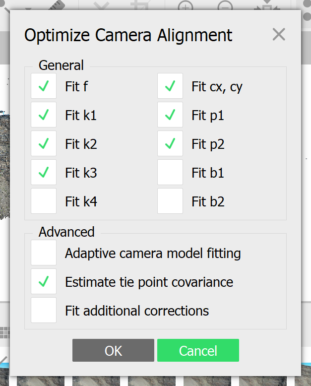
Fig. 12 The Optimize Camera Alignment dialog after opening it from the Tools menu. Make sure to enable Fit f, Fit k1-k3, Fit cx, cy, Fit p1-p2, and Estimate tie point covariance.#
Once processing is done, change the model view to show the Point Cloud Variance by following the instructions given in dialog. Lower values (=blue) are generally better and more constrained.
Fig. 13 Changing the view of your points and model to show errors and other things. Here we change our view to show Spare Point Covariance instead of RGB coloring.#
As the sparse cloud is the very first step in a long processing chain, we want to optimize it as much as possible. After all, bad quality in usually equals bad quality out. We will now conduct several optimizations to improve quality of the sparse cloud, implementing USGS [] recommendations that aim to reduce reconstruction uncertainty, improve projection accuracy, and lower the overall reprojection errors. Unlike shown below, the project sometimes benefits by having each of the steps repeated multiple times, rather than just once. Keep in mind, however, that running too many optimizations may also result in over-fitting of the data. That means that the model is no longer based on real input, but rather on the processing parameters (= not real!).
Make a backup for every step
Whenever you are about to perform a destructive action (i.e., “deleting” stuff), make sure to make a backup of the current state first. In Metashape this can be done by right clicking an object (e.g., Chunk, Points, etc.) and selecting the Duplicate… option. It usually takes a bit of time to complete, but the cost of not doing so is usually much, much higher!
Fig. 14 Making a backup duplicate of Chunk 1. To keep things simple, make sure to rename your copies; else you may end up with a Copy of Copy of Copy of Something…#
Use Python scripting
The following subsections may be automated through use of the built-in consol and Python code available through the Python snippets section.
Filtering by Reconstruction Uncertainty#
Once you’re ready (ahem, make a duplicate/backup first!), filter your Sparse points by their Reconstruction Uncertainty.
Fig. 15 The Gradual Selection dialog after opening it from the Model menu, here showing selections that are possible for the Sparse Point Cloud. A good value to use here is 10, though make sure you do not remove all points by doing so! After clicking OK, the left corner shows you how many points there are in total, followed by the number currently selected. A rule of thumb is to select no more than two-thirds to half of all points, and then delete these by pressing the Delete key on the keyboard.#
After deleting the selected points, it is important to once more optimize the alignment of your points. Do so by revisiting the Improve alignment step: Error Reduction-Optimization and Camera Calibration section.
Filtering by Projection accuracy#
This time, select the points based on their Projection accuracy, aiming for a final Projection accuracy of 3.
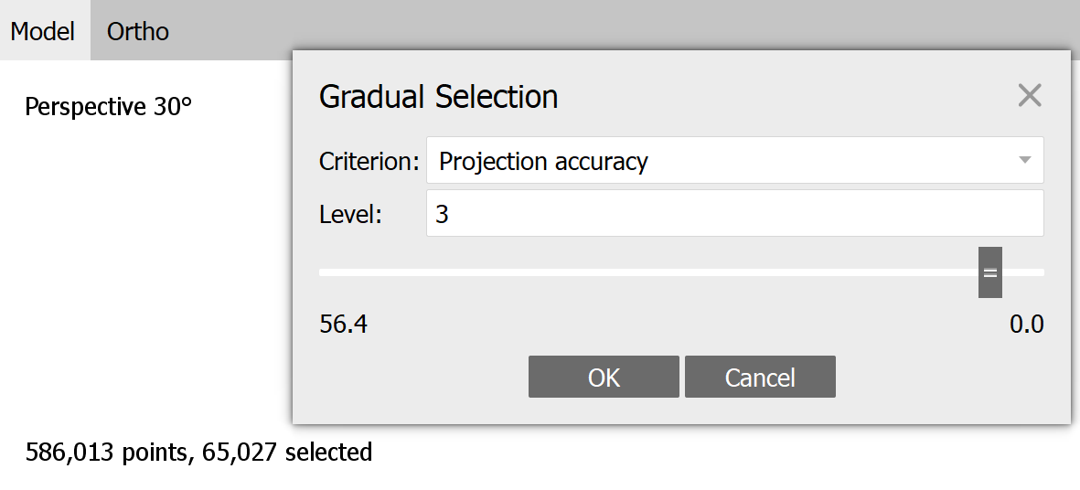
Fig. 16 The Gradual Selection dialog after opening it from the Model menu, here making a selection based on the projection accuracy parameter. A good value to use here is 3, though make sure you do not remove all points by doing so! After clicking OK, the left corner shows you how many points there are in total, followed by the number currently selected.#
Keep in mind that not all projects can tolerate the removal of points below 5, which is no problem as long as you document the values you have used. After deleting the selected points, it is important to once more optimize the alignment of your points. Do so by revisiting the Improve alignment step: Error Reduction-Optimization and Camera Calibration section.
Filtering by Reprojection Error#
Up next is to filter the points by their reprojection error, see dialog. A good value to use here is 0.3, though make sure you do not remove all points by doing so! As a rule of thumb, this final selection of points should leave you with approx. 10% of the points you started off with.
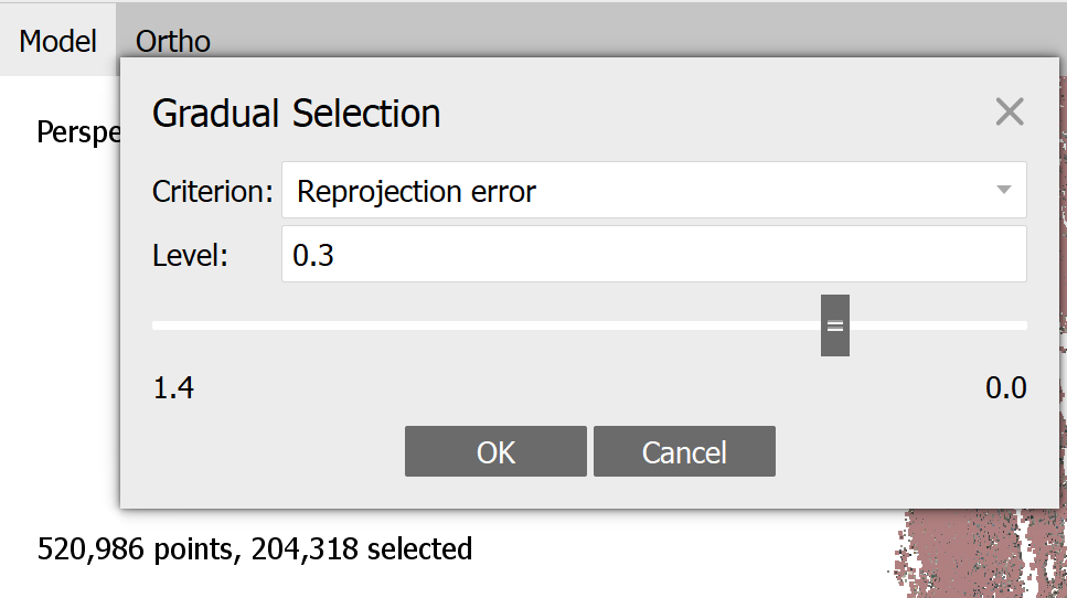
Fig. 17 The Gradual Selection dialog after opening it from the Model menu, here making a selection based on the reprojection error parameter. After clicking OK, the left corner shows you how many points there are in total, followed by the number currently selected.#
After deleting the selected points, it is important to runa final Optimize alignment step on your points. Do so by revisiting the Improve alignment step: Error Reduction-Optimization and Camera Calibration section.
Keep your duplicates
It is always a good idea to keep your duplicate backups of previous steps until you are fully done with them. They allow you to go back and write down important processing parameters, such as how many points were filtered during each step and which cutoff values you used during processing. Only once completely done should you remove these earlier attempts.
Build Point Cloud#
Based on the estimated camera positions, we can now estimate a dense point cloud by calculating depth information for each image.
Select Build Point Cloud from the Workflow menu. Once again you will be asked about the desired accuracy/quality. Keeping in mind what we discussed above, make sure to select Medium for the quality.
Also open up the Advanced section, and set Depth filtering to Mild. Make sure to always enable Calculate point confidence
Reuse depth maps can only be selected if depth maps have been previously calculated for the specified quality.
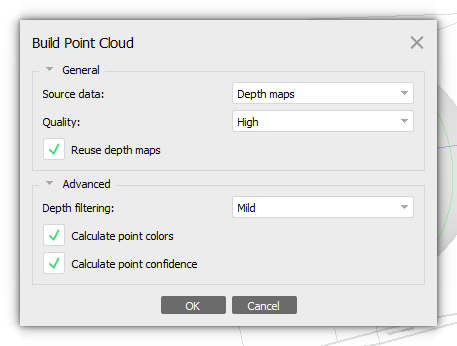
Fig. 18 The Build Point Cloud dialog after opening it from the Workflow menu. Reuse depth maps when avaialable. Always toggle Calculate Point Confidence.#
Once processing is done, you’ll be able to show the dense point cloud on the screen in the Model tab. If not, one can visualise the dense point cloud by clicking on the nine-dotted icon in the menu. Alternative, you could also visualise the point confidence. Do so by clicking the gray triangle next to the nine-dotted icon and selecting Point Cloud confidence. The colour coding (red = bad, blue = good) shows where the best confidence is found.
Point confidence
Point confidence shows how accurate a given point in the Point Cloud is. This is key to estimate whether the part we are interested in can be scientifically used for measurements and characterisation based on predefined criteria.
Point Cloud quality
While this tutorial suggests Medium to be used for the quality parameter, you should feel free to change this depending on the computational power at your disposal.
Selection by point confidence#
Save time - make backups
Make sure to always either backup your data before playing with it. This can be done by either backing up the entire project (Save as…) or by making a local copy of the data within the project. To do the latter, right click on the Workspace/Point Cloud (… points) and select Duplicate…. Following alterations to the duplicated data set, you can always switch back to the original by right clicking Workspace/Point Cloud (… points) and Set As Default.
There are various ways of cutting off parts of your Point Cloud. However, not all of them are scientifically repeatable - because let’s be honest, would you be able to exactly tell which of the points you removed from the data? No.
Luckily, Metashape allows selection and deletion of points by Point confidence. Proceed to Tools/Point Cloud in the menu and click on Filter by confidence…. The dialog that pops up allows you to set minimal and maximal confidences.
For example, try setting Min:50 and Max:255 to only show the Point Cloud points wth the highest confidence. After looking at the difference, reset the filter by clicking on Reset filter within the Tools/Point Cloud menu.
We will now use the method outlined above to filter out the lowest confidence interval (in this case, set Min:0 and Max:5). Proceed by selecting all the points shown in the Model tab. Do this by enabling the Rectangle Selection tool, found next to the mouse pointer icon in the menu. Then drag a rectangle selection and include all to-be-selected points currently visible. Delete the selected points by hitting the Del(ete) key on the keyboard.
Now reset the filter, and you’ll see that just the high-confidence part remains. :)
Scientific repeatability
Always write down the chosen confidence interval - repeatability depends on it!
Building a model#
We can use the point cloud to generate a polygonal model. While generating the Point Cloud, Agisoft Metashape simultaneously generated a set of depth maps (if chosen to save to the project). This is important as we can decide which of the two to use for building the model. Depth maps may lead to better results when dealing with a big number of minor details, but otherwise Point Clouds should be used as the source.
After selecting Build Model from the Workflow menu, you will be able to chose either in the dialog that pops up for Source data:.
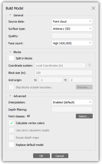
Fig. 19 The Build model dialog after opening it from the Workflow menu.#
Other important parameters here are the Quality and Face count parameters. These govern the quality of the generated model. Remember, however, that quality comes at a cost, so best to stick to Medium or lower to manage the exercise within the allocated of time…
Finally, feel free to enable the Calculate vertext colors to provide the model with some colour as well, otherwise it will be shown as a purple model.
Once generated, we can take a closer look at the model by clicking on the Tetrahedral icon next to the nine-dotted icon. Clicking on the gray triangle next to it, you see that the Model Textured is still grayed out. The next step involves generating a texture and placing this “image” onto the model - after which the Model Textured becomes selectable.
Depth maps
If depth maps do exist, and you decide to use them as the source data, then make sure to enable Reuse depth maps to save computational time!
Filtering the model#
Sometiems your model features blobs that are not connected to the main model. These can be easily (and scientifically!) removed through use of the Connected component filter, see dialog.
Fig. 20 Filtering the model based on the connected component size. This is a percentage of the largest component, which by default is 100.#
Select the model first!
The option may not be available if you have not selected the model data first, or not in the model view panel.
Texture building#
We can build the textures by clicking on the Build Texture command from the Workflow menu. While the dialog has many different parameters, the most important are highlighted in Fig. 21.
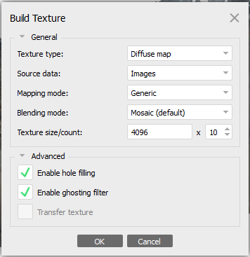
Fig. 21 The Build texture dialog after opening it from the Workflow menu.#
Here Texture size/count determines the quality of the texture. Keep in mind that anything over 16384 can very quickly lead to very, very large file sizes on your harddisk. On the other hand, anything less than 4096 is probably insufficient. For greatest compatibility, keep the Texture size at 4096, but increase the count to e.g. 5 or 10.
Publishing on V3Geo or Sketchfab
Publication guidelines for V3Geo specify that the Texture size must always be 4096. In addition, no fewer than 10 Texture count must be used. It is recommended to follow this even for SketchFab, as this setup generally results in a higher-quality look of the published model.
Generating a Tiled Model#
Sometimes the need arises to not only build a model, but also a Tiled Model. We can do this by selecting Build Tiled Model from the Workflow menu. Once again we can select the parameters for the processing step through the dialog that popped up.
The most import parameter here is the Pixel size (m), which should never be set than lower than the pixel size available to the model (= the default value shown when opening the dialog).
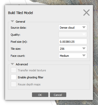
Fig. 22 The Build Tiled Model dialog after opening it from the Workflow menu.#
Build Digital Elevation Model (DEM)#
Digital Elevation Model (DEM) represents a surface model as a regular grid of height values. Select the Build DEM command from the Workflow menu. A dialog box will open to choose the parameters for building DEM.
To start, we need to check the Projection type:
Geographic : With the Geographic feature, you can select a geographic coordinate system either from the dropdown menu or enter the parameters for a customized system. It’s important to specify the coordinate system used for referencing the model. When exporting the results, it will be possible to project them onto a different geographic coordinate system.
Planar: You can project a DEM onto a plane of your choice. You can select the projection plane and orientation of the resulting DEM.
Cylindrical: This parameter enables the projection of DEM onto a cylindrical surface. The height value is determined by measuring the distance between the model surface and the cylindrical surface.
Agisoft Metashape allows the DEM generation based on the point cloud or model. It is recommended to use Point Cloud as the source data since it provides more accurate results and faster processing. You can generate elevation data results from depth maps or a tie point cloud. If you need the DEM to follow the polygonal model precisely or if the point cloud hasn’t been reconstructed, you can use the Model and Tiled Model options.
We suggest keeping the interpolation parameter Disabled for accurate reconstruction results since only areas corresponding to point cloud or polygonal points are reconstructed. Usually, this method is recommended for Model and Tiled Model data source.
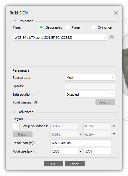
Fig. 23 The Build DEM dialog after opening it from the Workflow menu. The Geographic type is used to generate the DEM in a known geographic projection (here shown for EPSG:32633).#
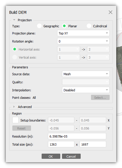
Fig. 24 The Build DEM dialog after opening it from the Workflow menu. The Planar type is used to generate the DEM in a local coordinate system based on the specified Projection plane. This is useful for generating high-resolution cross-section views of the model.#
Once the DEM generation process is complete, you can view the reconstructed model in Ortho view by clicking the Basemap button on the Toolbar.
Build Orthomosaic#
Building and exporting an orthomosaic is normally used for generation of high resolution imagery based on the source photos and reconstructed model.
Note
The Build Orthomosaic procedure is only possible for projects saved in .PSX format that have existing model or DEM chunks.
To start building and orthomosaic, select Build Orthomosaic command from the Workflow menu.
To begin, you have to select the Projection parameter.
Geographic projectionis often used for aerial photogrammetric surveys.
Planar projection is helpful when working with models that have vertical surfaces, such as vertical digital outcrop models.
Cylindrical projection can help reduce distortions when projecting cylindrical objects like tubes, rounded towers, or tunnels.
To generate an accurate orthomosaic, we advise selecting Model as the desired surface. For complete coverage, we recommend selecting the Enable hole filling option under Blending mode to fill in any empty areas of the mosaic.
The suggested Pixel size (m) will be based on the average ground sampling resolution of the original images. Using the surface size and input pixel size, the total size of the orthomosaic (measured in pixels) will be calculated and displayed at the bottom of the dialogue box.
Note
You can store multiple Orthomosaic instances in a single chunk. To save the current Orthomosaic and create a new one in the same chunk, right-click on the Orthomosaic and uncheck the Set as default option. If you want to save the current Orthomosaic and make a copy for editing, right-click on the Orthomosaic and select Duplicate.
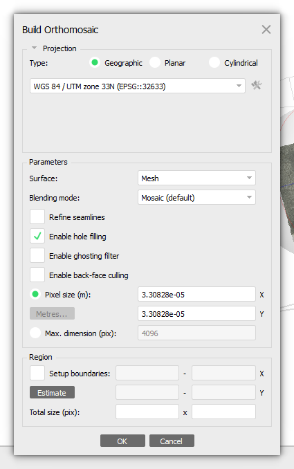
Fig. 25 The Build Orthomosaic dialog after opening it from the Workflow menu. The Geographic type is used to generate the Orthomosaic in a known geographic projection (here shown for EPSG:32633).#
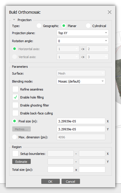
Fig. 26 The Build Orthomosaic dialog after opening it from the Workflow menu. The Planar type is used to generate the orthomosaic in a local coordinate system based on the specified Projection plane. This is useful for generating high-resolution cross-section views of the model.#
Generated orthomosaic can be reviewed in Ortho mode similar to the digital elevation model. It can be opened in this view mode by double-clicking on the orthomosaic label in the Workspace pane.
Documenting processing parameters#
While each of the previous steps has been important in generating the models, perhaps the most important aspect of processing is to document the taken processing steps and their parameters. Metashape automatically keeps track and stores all Workflow actions that the project has undergone. There are two ways of documenting and showing these parameters.
What about manual alterations?
Sadly, the processing report does not include manual changes made to e.g. the point or Point Cloud. This means that to be truly scientifically grounded and repeatable, you should refrain from doing such alterations manually. Instead, rely on e.g. the point confidence to make edits (and always report the chosen parameters).
Processing report#
The first, and perhaps most important, is to generate a processing report. Proceed to File/Export in the menu bar and select Generate Report…. Provide the desired Title and description, then proceed by clicking OK. Store the report alongside the Metashape project in the same directory.
Note
The procedure listed above should always be implemented in your workflows, with the output stored together with the raw data (e.g., images) and Metashape project files. Make this a habit :)
Exercise 2
You’ll find key metadata within the generated processing_report.pdf that has to be submitted as part of the second session’s assignment. Have a look and familiarise yourself with it.
In-programme parameters#
One does not always need to export the processing report to obtain the overview of parameters. Handily, Metashape also provides an overview within the Workspace panel after having selected an item in the chunk. An example of this is depicted in Fig. 27.
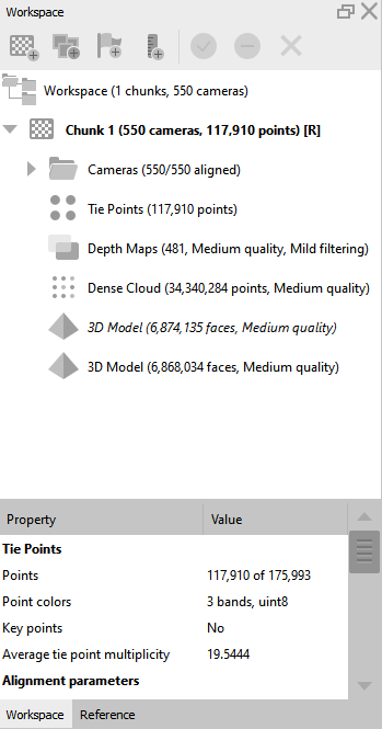
Fig. 27 An example of the internal Workspace panel, including the parameters and processing metadata that is available from within the Metashape project interface.#
Tip
The above is just a very generalised approach to SfM-photogrammetry that outlines the basic steps to be taken from photo acquisition to model generation. In many cases the chosen parameters can (and should!) be changed to match the given circumstances. That said, the Photo alignment step should always be conducted at the highest setting possible (considering computational power available). Furthermore, one should always document each and every processing step performed - manually cutting and editing part of the model is therefore not encouraged as this remains (for now) difficult to document.
Record video#
Agisoft Metashape allows the creation of a camera track. To do so you have to add viewpoints.
Note
To display the camera track path, select Model > Show/Hide items > Show animation.
Fig. 28 Display the Animation menu.#
To create a viewpoint, first set up the scene in the Model view according to how you want it to appear in the animation. Next, click on the Append button located on the Animation pane to add the viewpoint to the current camera track.
If you need to change the position of the viewpoints along the camera track, simply use your left mouse button to drag the waypoints.
After creating the waypoints, you need to record the video according to the camera track you’ve created. To do this, click the Capture button on the Animation pane toolbar and choose the desired export parameters, such as video resolution, compression type, and frame rate in the Capture Video dialog. Once you’ve made your selections, click the OK button to save the video as a separate file.
Fig. 29 Creation of an animation with two waypoints over 5 seconds.#
Publishing#
The Publish 3D models page explains how to export your 3D model and how to best upload it to online technical solutions like Sketchfab.